Gamma Survey

Built using Zelig version 5.1.0.90000

Gamma Regression for Continuous, Positive Dependent Variables with gamma.survey.

Use the gamma regression model if you have a positive-valued dependent variable such as the number of years a parliamentary cabinet endures, or the seconds you can stay airborne while jumping. The gamma distribution assumes that all waiting times are complete by the end of the study (censoring is not allowed).

Syntax

With reference classes:

z5 <- zgammasurvey$new()
z5$zelig(Y ~ X1 + X ~ X, weights = w, data = mydata)
z5$setx()
z5$sim()

With the Zelig 4 compatibility wrappers:

z.out <- zelig(Y ~ X1 + X2, model = "gamma.survey", weights = w, data = mydata)
x.out <- setx(z.out)
s.out <- sim(z.out, x = x.out, x1 = NULL)

Examples

Example 1: User has Existing Sample Weights

Attach sample data and variable names:

data(api, package="survey")

In this example, we will estimate a model using the percentages of students who receive subsidized lunch and an indicator for whether schooling is year-round to predict California public schools’ academic performance index scores:

z.out1 <- zelig(api00 ~ meals + yr.rnd, model = "gamma.survey",
                weights = ~pw, data = apistrat)

## Warning: Supplied weights argument is not a vector or a variable name in the dataset, and will be ignored.

summary(z.out1)

## Model: 
## 
## Call:
## z5$zelig(formula = api00 ~ meals + yr.rnd, data = apistrat, weights = ~pw)
## 
## Survey design:
## survey::svydesign(data = data, ids = ids, probs = probs, strata = strata, 
##     fpc = fpc, nest = nest, check.strata = check.strata, weights = localWeights)
## 
## Coefficients:
##              Estimate Std. Error t value Pr(>|t|)
## (Intercept) 1.162e-03  1.645e-05   70.66   <2e-16
## meals       7.859e-06  4.363e-07   18.01   <2e-16
## yr.rndYes   2.807e-05  4.456e-05    0.63    0.529
## 
## (Dispersion parameter for Gamma family taken to be 0.01251498)
## 
## Number of Fisher Scoring iterations: 4
## 
## Next step: Use 'setx' method

Set explanatory variables to their default (mean/mode) values, and set a high (80th percentile) and low (20th percentile) value for “meals,” the percentage of students who receive subsidized meals:

x.low <- setx(z.out1, meals= quantile(apistrat$meals, 0.2))
x.high <- setx(z.out1, meals= quantile(apistrat$meals, 0.8))

Generate first differences for the effect of high versus low “meals” on academic performance:

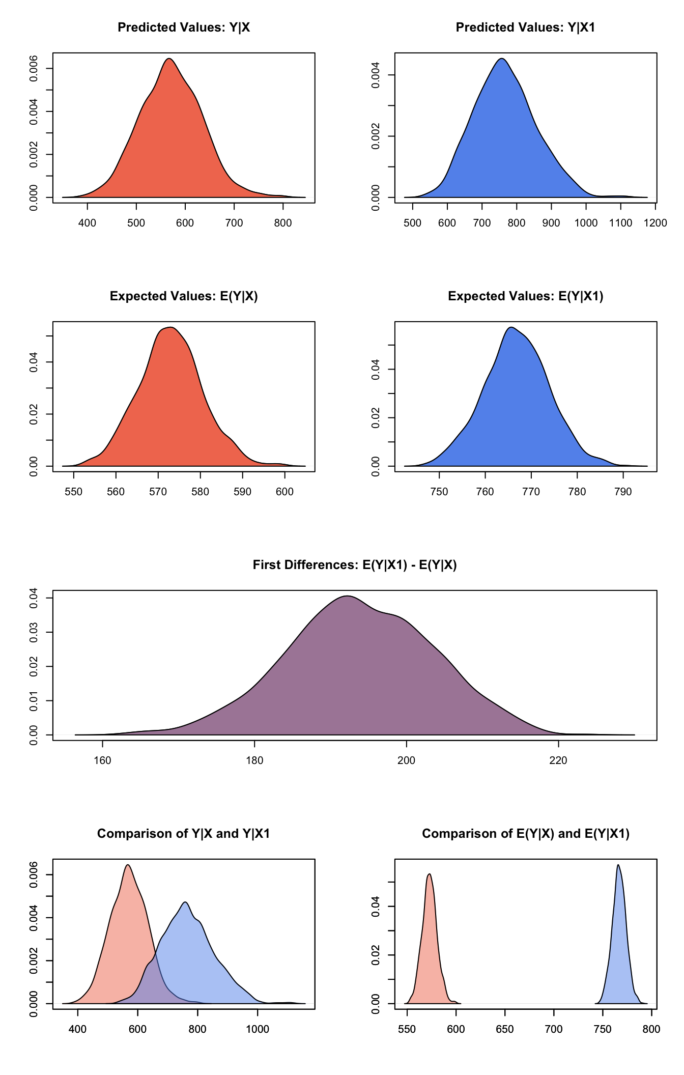
s.out1 <- sim(z.out1, x=x.high, x1=x.low)
summary(s.out1)

## 
##  sim x :
##  -----
## ev
##          mean       sd      50%     2.5%   97.5%
## [1,] 572.9882 7.590812 573.0584 558.7091 588.147
## pv
##          mean       sd      50%     2.5%    97.5%
## [1,] 571.2371 63.46556 569.7145 450.9827 699.9748
## 
##  sim x1 :
##  -----
## ev
##         mean       sd      50%     2.5%    97.5%
## [1,] 766.822 7.037657 766.6942 752.9023 780.7117
## pv
##          mean       sd      50%     2.5%    97.5%
## [1,] 766.3199 89.52293 762.2232 605.8467 947.5068
## fd
##          mean      sd      50%     2.5%    97.5%
## [1,] 193.8338 9.67774 193.6547 174.5175 212.2267

Generate a second set of fitted values and a plot:

plot(s.out1)

Graphs of Quantities of Interest for Gamma Survey

Example 2: User has Details about Complex Survey Design (but not sample weights)

Suppose that the survey house that provided the dataset excluded probability weights but made other details about the survey design available. We can still estimate a model without probability weights that takes instead variables that identify each the stratum and/or cluster from which each observation was selected and the size of the finite sample from which each observation was selected.

z.out2 <- zelig(api00 ~ meals + yr.rnd, model = "gamma.survey",
                strata=~stype, fpc=~fpc, data = apistrat)
summary(z.out2)

## Model: 
## 
## Call:
## z5$zelig(formula = api00 ~ meals + yr.rnd, data = apistrat, strata = ~stype, 
##     fpc = ~fpc)
## 
## Survey design:
## survey::svydesign(data = data, ids = ids, probs = probs, strata = strata, 
##     fpc = fpc, nest = nest, check.strata = check.strata, weights = localWeights)
## 
## Coefficients:
##              Estimate Std. Error t value Pr(>|t|)
## (Intercept) 1.162e-03  1.472e-05  78.980   <2e-16
## meals       7.859e-06  4.276e-07  18.380   <2e-16
## yr.rndYes   2.807e-05  4.392e-05   0.639    0.523
## 
## (Dispersion parameter for Gamma family taken to be 0.01251498)
## 
## Number of Fisher Scoring iterations: 4
## 
## Next step: Use 'setx' method

Note that these results are identical to the results obtained when pre-existing sampling weights were used. When sampling weights are omitted, Zelig estimates them automatically for “gamma.survey” models based on the user-defined description of sampling designs. If no description is present, the default assumption is equal probability sampling.

The methods setx()`` andsim()can then be run onz.out2` in the same fashion described in Example 1.

Example 3: User has Replicate Weights

Suppose that the survey house that published these data withheld details about the survey design and instead published replication weights.

For the purpose of illustration, create a set of jk1 replicate weights:

library("survey")

## Loading required package: grid

## Loading required package: Matrix

## 
## Attaching package: 'survey'

## The following object is masked from 'package:graphics':
## 
##     dotchart

jk1reps <- jk1weights(psu=apistrat$dnum)

Estimate the model regressing api00 on the “meals” “yr.rnd” variables.

z.out3 <- zelig(api00 ~ meals + yr.rnd, model = "gamma.survey",
      data = apistrat, repweights=jk1reps$weights,
      type="JK1")
summary(z.out3)

## Model: 
## 
## Call:
## z5$zelig(formula = api00 ~ meals + yr.rnd, data = apistrat, repweights = jk1reps$weights, 
##     type = "JK1")
## 
## Survey design:
## survey::svydesign(data = data, ids = ids, probs = probs, strata = strata, 
##     fpc = fpc, nest = nest, check.strata = check.strata, weights = localWeights)
## 
## Coefficients:
##               Estimate Std. Error t value Pr(>|t|)
## (Intercept)  1.210e-03  1.858e-05  65.146   <2e-16
## meals        7.868e-06  4.658e-07  16.891   <2e-16
## yr.rndYes   -6.263e-06  4.639e-05  -0.135    0.893
## 
## (Dispersion parameter for Gamma family taken to be 0.01458664)
## 
## Number of Fisher Scoring iterations: 4
## 
## Next step: Use 'setx' method

Set the explanatory variable “meals” at high and low values

x.low <- setx(z.out3, meals= quantile(apistrat$meals, 0.2))
x.high <- setx(z.out3, meals= quantile(apistrat$meals, 0.8))

Generate first differences for the effect of the high versus low concentrations of poverty on school performance

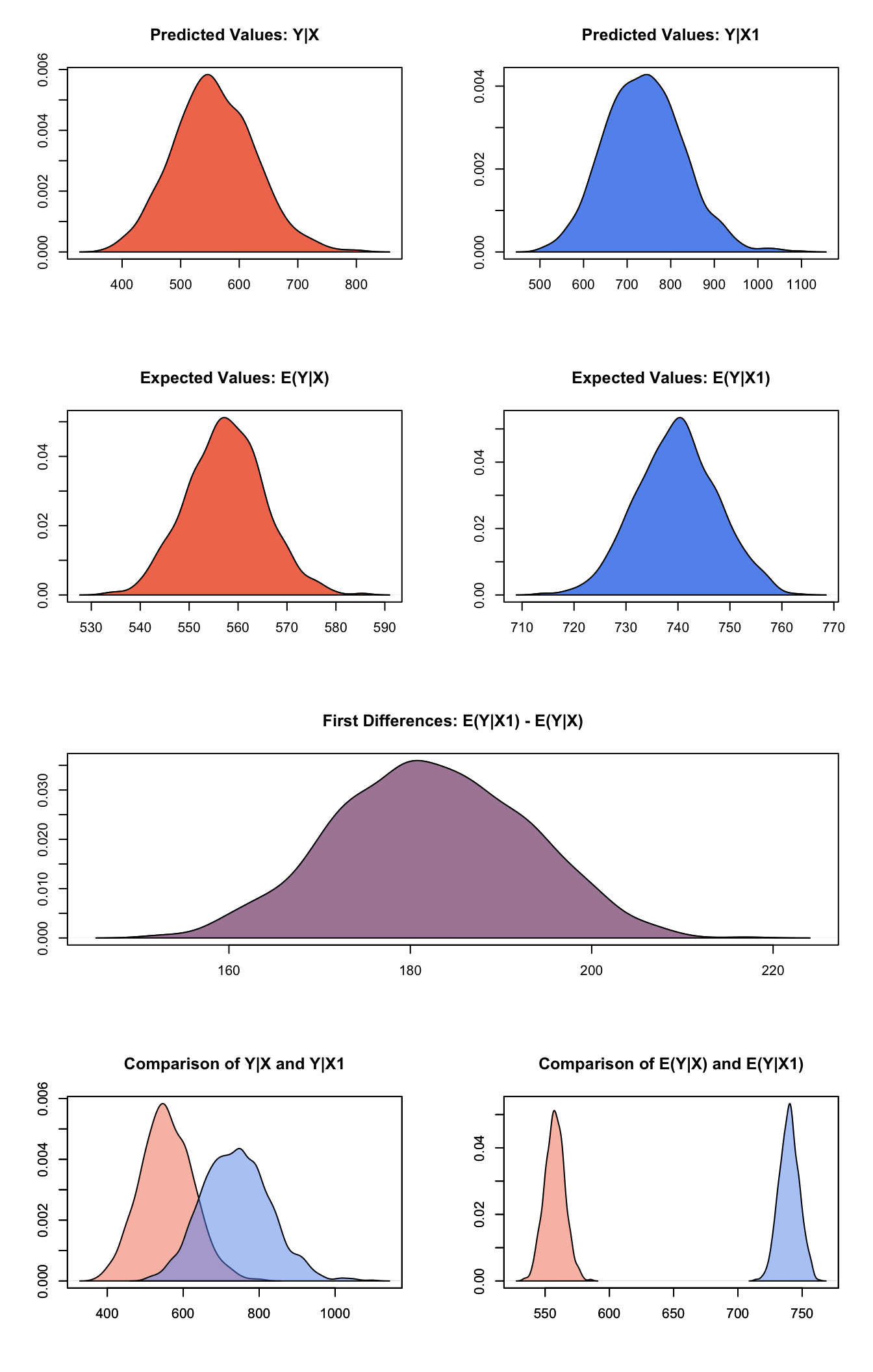
s.out3 <- sim(z.out3, x=x.high, x1=x.low)
summary(s.out3)

## 
##  sim x :
##  -----
## ev
##          mean      sd      50%     2.5%    97.5%
## [1,] 557.5092 7.82784 557.5356 542.6838 573.5134
## pv
##          mean       sd      50%     2.5%    97.5%
## [1,] 557.1642 69.00516 553.7461 427.6548 701.4656
## 
##  sim x1 :
##  -----
## ev
##          mean       sd     50%     2.5%    97.5%
## [1,] 739.8227 7.723049 739.909 725.2179 755.3492
## pv
##          mean       sd      50%     2.5%    97.5%
## [1,] 739.4973 88.68498 738.1387 573.5824 916.5185
## fd
##          mean       sd      50%     2.5%   97.5%
## [1,] 182.3135 10.45998 182.1638 162.0031 201.874

Generate a second set of fitted values and a plot:

plot(s.out3)

The user should also refer to the gamma model demo, since gamma.survey models can take many of the same options as gamma models.

Model

The Gamma distribution with scale parameter $\alpha$ has a stochastic component:

$$ \[\begin{aligned} Y &\sim& \textrm{Gamma}(y_i \mid \lambda_i, \alpha) \\ f(y) &=& \frac{1}{\alpha^{\lambda_i} \, \Gamma \lambda_i} \, y_i^{\lambda_i - 1} \exp -\left\{ \frac{y_i}{\alpha} \right\}\end{aligned}\]

for $\alpha, \lambda_i, y_i > 0$.

The systematic component is given by

\[ \lambda_i = \frac{1}{x_i \beta} \]

Quantities of Interest

The expected values (qi$ev) are simulations of the mean of the stochastic component given draws of $\alpha$ and $\beta$ from their posteriors:

\[ E(Y) = \alpha \lambda_i. \]

The predicted values (qi$pr) are draws from the gamma distribution for each given set of parameters $(\alpha, \lambda_i)$.
If x1 is specified, sim() also returns the differences in the expected values (qi$fd),

\[ E(Y \mid x_1) - E(Y \mid x) \]

In conditional prediction models, the average expected treatment effect (att.ev) for the treatment group is

\[ \frac{1}{\sum_{i=1}^n t_i}\sum_{i:t_i=1}^n \left\{ Y_i(t_i=1) - E[Y_i(t_i=0)] \right\}, \]

where $t_i$ is a binary explanatory variable defining the treatment ($t_i=1$) and control ($t_i=0$) groups. Variation in the simulations are due to uncertainty in simulating $E[Y_i(t_i=0)]$, the counterfactual expected value of $Y_i$ for observations in the treatment group, under the assumption that everything stays the same except that the treatment indicator is switched to $t_i=0$.

In conditional prediction models, the average predicted treatment effect (att.pr) for the treatment group is

\[ \frac{1}{\sum_{i=1}^n t_i}\sum_{i:t_i=1}^n \left\{ Y_i(t_i=1) - \widehat{Y_i(t_i=0)} \right\}, \]

where $t_i$ is a binary explanatory variable defining the treatment ($t_i=1$) and control ($t_i=0$) groups. Variation in the simulations are due to uncertainty in simulating $\widehat{Y_i(t_i=0)}$, the counterfactual predicted value of $Y_i$ for observations in the treatment group, under the assumption that everything stays the same except that the treatment indicator is switched to $t_i=0$.

Output Values

The Zelig object stores fields containing everything needed to rerun the Zelig output, and all the results and simulations as they are generated. In addition to the summary commands demonstrated above, some simply utility functions (known as getters) provide easy access to the raw fields most commonly of use for further investigation.

In the example above z.out$get_coef() returns the estimated coefficients, z.out$get_vcov() returns the estimated covariance matrix, and z.out$get_predict() provides predicted values for all observations in the dataset from the analysis.

2017-05-04