Built using Zelig version 5.1.0.90000

Instrumental Variable Regression (2 Stage Least Squares) for Continuous Dependent Variables with ivreg.

Syntax

With Zelig 5 reference classes:

z5 <- zls$new()
z5$zelig(Y ~ X1 + X2 | Z1 + Z2 + Z3, weights = w, data = mydata)
z5$setx()
z5$sim()

Note that | separates the regressors (e.g. X1 and X2) from the instruments (e.g. Z1, Z2, Z3).

With the Zelig 4 compatibility wrappers:

z.out <- zelig(Y ~ X1 + X2 | Z1 + Z2 + Z3, model = "ivreg", weights = w,
               data = mydata)
x.out <- setx(z.out)
s.out <- sim(z.out, x = x.out)

Examples

Load Zelig and other packages used in the example:

library(Zelig)
library(dplyr) # for the pipe operator %>%

Before estimating the model, let’s attach the example data and make some transformations to it. Notably, zivreg does not currently support logging regressors in the zelig call. To get around this, we simply find the logged values before estimating the model:

# load and transform data
data("CigarettesSW")
CigarettesSW$rprice <- with(CigarettesSW, price/cpi)
CigarettesSW$rincome <- with(CigarettesSW, income/population/cpi)
CigarettesSW$tdiff <- with(CigarettesSW, (taxs - tax)/cpi)

# log second stage independent variables, as logging internally for ivreg is
# not currently supported
CigarettesSW$log_rprice <- log(CigarettesSW$rprice)
CigarettesSW$log_rincome <- log(CigarettesSW$rincome)

Now we can estimate the model and summarize the coefficients:

z.out1 <- zelig(log(packs) ~ log_rprice + log_rincome |
                    log_rincome + tdiff + I(tax/cpi),
                    data = CigarettesSW, subset = year == "1995",
                    model = "ivreg")

summary(z.out1)

## Model: 
## 
## Call:
## z5$zelig(formula = log(packs) ~ log_rprice + log_rincome | log_rincome + 
##     tdiff + I(tax/cpi), data = CigarettesSW, subset = year == 
##     "1995")
## 
## Residuals:
##        Min         1Q     Median         3Q        Max 
## -0.6006931 -0.0862222 -0.0009999  0.1164699  0.3734227 
## 
## Coefficients:
##             Estimate Std. Error t value Pr(>|t|)
## (Intercept)   9.8950     1.0586   9.348 4.12e-12
## log_rprice   -1.2774     0.2632  -4.853 1.50e-05
## log_rincome   0.2804     0.2386   1.175    0.246
## 
## Residual standard error: 0.1879 on 45 degrees of freedom
## Multiple R-Squared: 0.4294,  Adjusted R-squared: 0.4041 
## Wald test: 13.28 on 2 and 45 DF,  p-value: 2.931e-05 
## 
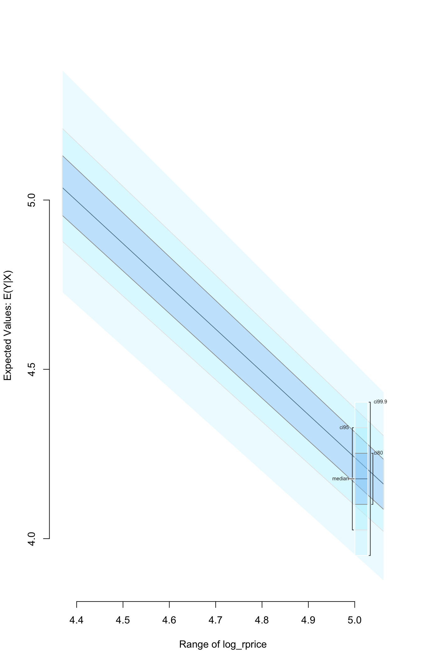
## Next step: Use 'setx' method

We can then simulate and plot the expected value of the log of the packs response variable across the range of the observed rprice regressor values:

z.out1 %>% setx(log_rprice = range(log(CigarettesSW$rprice))) %>%
    sim() %>%
    plot()

To conduct standard diagnostic tests on the estimated model using functionality in the AER package, exatract the fitted model object with the from_zelig_model() function.

Model

Let \(Y_i\) be the continuous dependent variable for observation \(i\).

See also

ivreg is from Christian Kleiber and Achim Zeileis (2008). Applied Econometrics with R. New York: Springer-Verlag. ISBN 978-0-387-77316-2. URL https://CRAN.R-project.org/package=AER. For more information use ?AER::ivreg.

Greene, W. H. (1993) Econometric Analysis, 2nd ed., Macmillan.