Ordered Logistic Regression

Built using Zelig version 5.1.0.90000

Ordinal Logistic Regression for Ordered Categorical Dependent Variables with ologit in ZeligChoice.

Use the ordinal logit regression model if your dependent variable is ordered and categorical, either in the form of integer values or character strings.

Syntax

First load packages:

library(zeligverse)

With reference classes:

z5 <- zologit$new()
z5$zelig(as.factor(Y) ~ X1 + X2, data = mydata)
z5$setx()
z5$sim()

With the Zelig 4 compatibility wrappers:

z.out <- zelig(as.factor(Y) ~ X1 + X23,
               model = "ologit", data = mydata)
x.out <- setx(z.out)
s.out <- sim(z.out, x = x.out, x1 = NULL)

If Y takes discrete integer values, the as.factor() command will order automatically order the values. If Y takes on values composed of character strings, such as “strongly agree”, “agree”, and “disagree”, as.factor() will order the values in the order in which they appear in Y. You will need to replace your dependent variable with a factored variable prior to estimating the model through zelig(). See below for more details.

Example

Creating An Ordered Dependent Variable

Load the sample data:

data(sanction)

Create an ordered dependent variable:

sanction$ncost <- factor(sanction$ncost, ordered = TRUE,
                         levels = c("net gain", "little effect", "modest loss", "major loss"))

Estimate the model:

z.out <- zelig(ncost ~ mil + coop, model = "ologit",
               data = sanction)

Summarize estimated paramters:

summary(z.out)

## Model: 
## Call:
## z5$zelig(formula = ncost ~ mil + coop, data = sanction)
## 
## Coefficients:
##          Value Std. Error   t value
## mil  -0.001308     0.7315 -0.001787
## coop  1.040545     0.2624  3.966071
## 
## Intercepts:
##                           Value   Std. Error t value
## net gain|little effect     1.2604  0.4816     2.6173
## little effect|modest loss  3.9364  0.6984     5.6364
## modest loss|major loss     5.6088  0.8994     6.2364
## 
## Residual Deviance: 153.0708 
## AIC: 163.0708 
## Next step: Use 'setx' method

Set the explanatory variables to their observed values:

x.out <- setx(z.out)

Simulate fitted values given x.out and view the results:

s.out <- sim(z.out, x = x.out)

summary(s.out)

## 
##  sim x :
##  -----
## ev
##                     mean         sd        50%         2.5%     97.5%
## net gain      0.34984401 0.05554039 0.34639060 2.487219e-01 0.4583356
## little effect 0.49436527 0.15173278 0.52247456 1.630364e-01 0.7113469
## modest loss   0.08310624 0.06974727 0.07047300 8.954845e-06 0.2441367
## major loss    0.07268448 0.11024066 0.01797867 6.759908e-09 0.3843584
## pv
##       mean        sd 50% 2.5% 97.5%
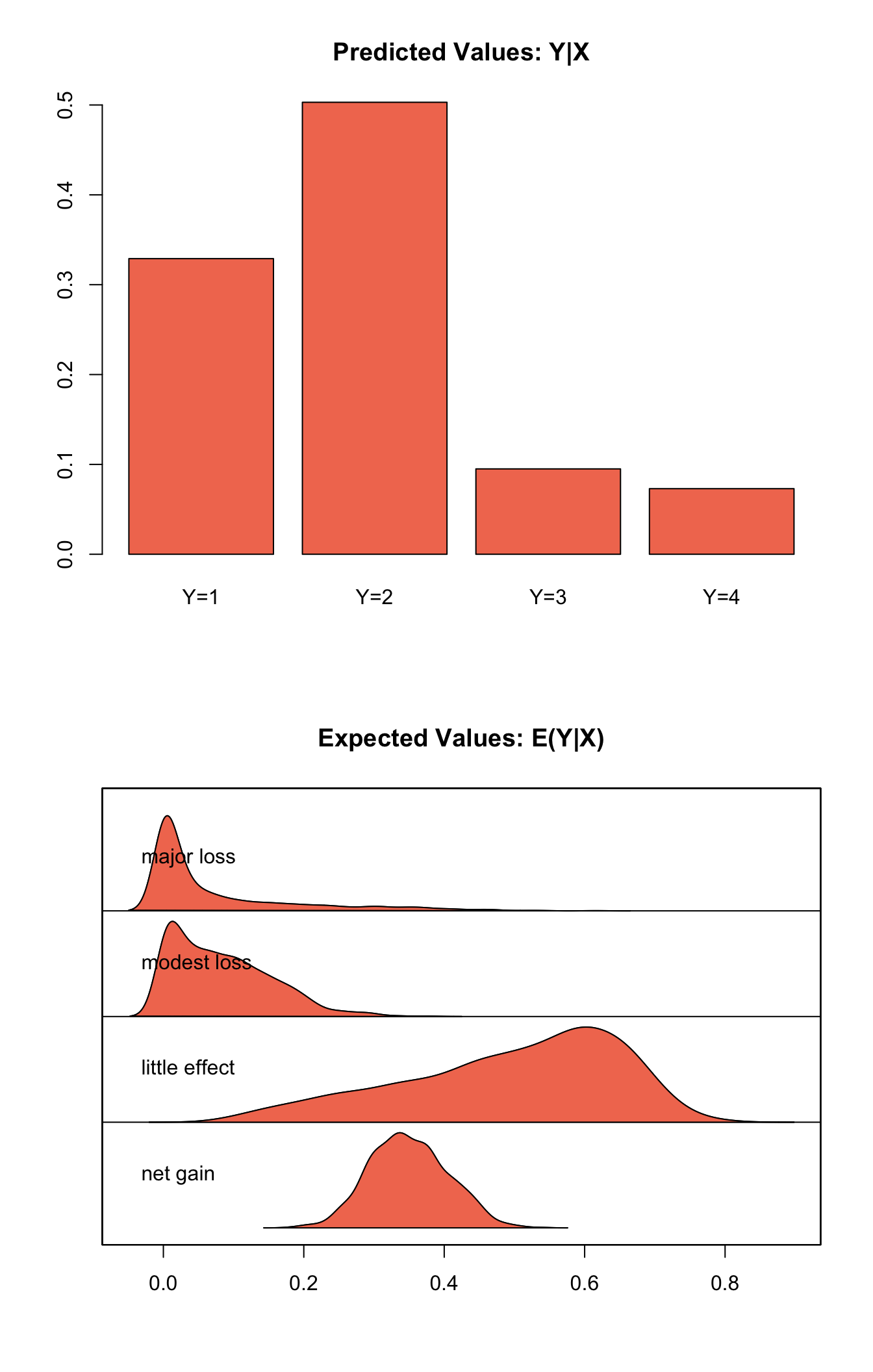
## [1,] 1.912 0.8420006   2    1     4

plot(s.out)

Graphs of Quantities of Interest for Ordered Logit

First Differences

Using the sample data sanction, estimate the empirical model and returning the coefficients:

z.out <- zelig(as.factor(cost) ~ mil + coop, model = "ologit",
               data = sanction)

summary(z.out)

## Model: 
## Call:
## z5$zelig(formula = as.factor(cost) ~ mil + coop, data = sanction)
## 
## Coefficients:
##          Value Std. Error   t value
## mil  -0.001308     0.7315 -0.001787
## coop  1.040545     0.2624  3.966071
## 
## Intercepts:
##     Value   Std. Error t value
## 1|2  1.2604  0.4816     2.6173
## 2|3  3.9364  0.6984     5.6364
## 3|4  5.6088  0.8994     6.2364
## 
## Residual Deviance: 153.0708 
## AIC: 163.0708 
## Next step: Use 'setx' method

Set the explanatory variables to their means, with coop set to 1 (the lowest value) in the baseline case and set to 4 (the highest value) in the alternative case:

x.low <- setx(z.out, coop = 1)
x.high <- setx(z.out, coop = 4)

Generate simulated fitted values and first differences, and view the results:

s.out2 <- sim(z.out, x = x.low, x1 = x.high)
summary(s.out2)

## 
##  sim x :
##  -----
## ev
##         mean         sd         50%         2.5%     97.5%
## 1 0.54917451 0.06893764 0.554228380 4.045219e-01 0.6766984
## 2 0.35680710 0.08084648 0.365391027 1.588826e-01 0.4926123
## 3 0.04917874 0.04747929 0.035837476 4.669180e-05 0.1653661
## 4 0.04483964 0.07645269 0.008156036 1.651239e-08 0.2684673
## pv
##       mean        sd 50% 2.5% 97.5%
## [1,] 1.639 0.8302821   1    1     4
## 
##  sim x1 :
##  -----
## ev
##         mean         sd        50%         2.5%     97.5%
## 1 0.06069958 0.03818996 0.05230804 1.571215e-02 0.1581855
## 2 0.45999341 0.28308893 0.40430236 8.115931e-02 0.9742038
## 3 0.23185009 0.15555495 0.21144726 3.938958e-03 0.5790817
## 4 0.24745692 0.24977115 0.15698150 1.107668e-06 0.7575716
## pv
##       mean        sd 50% 2.5% 97.5%
## [1,] 2.708 0.9041867   3    1     4
## fd
##         mean         sd         50%          2.5%      97.5%
## 1 -0.4884749 0.08412112 -0.49370652 -6.361015e-01 -0.3113523
## 2  0.1031863 0.24730317  0.02323077 -2.201819e-01  0.6054704
## 3  0.1826713 0.14699749  0.16595410 -1.458031e-02  0.5036310
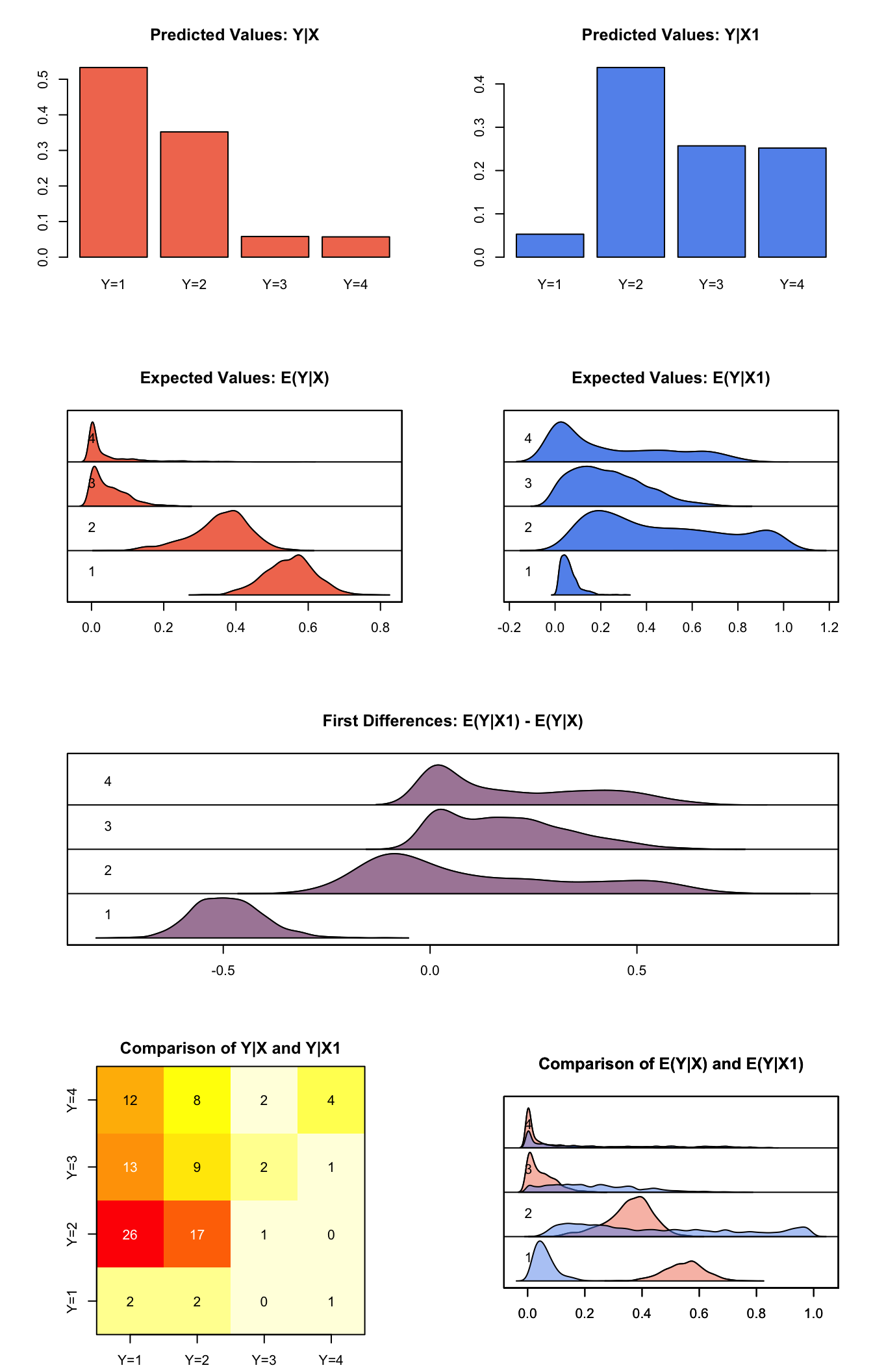
## 4  0.2026173 0.19285116  0.14503734  1.087602e-06  0.5822996

plot(s.out2)

Graphs of Quantities of Interest for Ordered Logit

Model

Let $Y_i$ be the ordered categorical dependent variable for observation $i$ that takes one of the integer values from $1$ to $J$ where $J$ is the total number of categories.

The stochastic component begins with an unobserved continuous variable, $Y^*_i$, which follows the standard logistic distribution with a parameter $\mu_i$,

\[ Y_i^* \; \sim \; \textrm{Logit}(y_i^* \mid \mu_i), \]

to which we add an observation mechanism

\[ Y_i \; = \; j \quad {\rm if} \quad \tau_{j-1} \le Y_i^* \le \tau_j \quad {\rm for} \quad j=1,\dots,J. \]

where $\tau_l$ (for $l=0,\dots,J$) are the threshold parameters with [_l]( _m[ for all $l](m$ and $\tau_0=-\infty$ and $\tau_J=\infty$.

The systematic component has the following form, given the parameters $\tau_j$ and $\beta$, and the explanatory variables $x_i$:

\[ \Pr(Y \le j) \; = \; \Pr(Y^* \le \tau_j) \; = \frac{\exp(\tau_j - x_i \beta)}{1+\exp(\tau_j -x_i \beta)}, \]

which implies:

\[ \pi_{j} \; = \; \frac{\exp(\tau_j - x_i \beta)}{1 + \exp(\tau_j - x_i \beta)} - \frac{\exp(\tau_{j-1} - x_i \beta)}{1 + \exp(\tau_{j-1} - x_i \beta)}. \]

Quantities of Interest

The expected values (qi$ev) for the ordinal logit model are simulations of the predicted probabilities for each category:

\[ E(Y = j) \; = \; \pi_{j} \; = \; \frac{\exp(\tau_j - x_i \beta)} {1 + \exp(\tau_j - x_i \beta)} - \frac{\exp(\tau_{j-1} - x_i \beta)}{1 + \exp(\tau_{j-1} - x_i \beta)}, \]

given a draw of $\beta$ from its sampling distribution.

The predicted value (qi$pr) is drawn from the logit distribution described by $\mu_i$, and observed as one of $J$ discrete outcomes.
The difference in each of the predicted probabilities (qi$fd) is given by

\[ \Pr(Y=j \mid x_1) \;-\; \Pr(Y=j \mid x) \quad {\rm for} \quad j=1,\dots,J. \]

In conditional prediction models, the average expected treatment effect (att.ev) for the treatment group is

\[ \frac{1}{n_j}\sum_{i:t_i=1}^{n_j} \left\{ Y_i(t_i=1) - E[Y_i(t_i=0)] \right\}, \]

where $t_{i}$ is a binary explanatory variable defining the treatment ($t_{i}=1$) and control ($t_{i}=0$) groups, and $n_j$ is the number of treated observations in category $j$.

In conditional prediction models, the average predicted treatment effect (att.pr) for the treatment group is

\[ \frac{1}{n_j}\sum_{i:t_i=1}^{n_j} \left\{ Y_i(t_i=1) - \widehat{Y_i(t_i=0)} \right\}, \]

where $t_{i}$ is a binary explanatory variable defining the treatment ($t_{i}=1$) and control ($t_{i}=0$) groups, and $n_j$ is the number of treated observations in category $j$.

Output Values

The output of each Zelig command contains useful information which you may view. For example, if you run z.out <- zelig(y ~ x, model = ologit, data), then you may examine the available information in z.out by using names(z.out), see the coefficients by using z.out$coefficients, and a default summary of information through summary(z.out). Other elements available through the $ operator are listed below.

From the zelig() output object z.out, you may extract:
coefficients: parameter estimates for the explanatory variables.
zeta: a vector containing the estimated class boundaries $\tau_j$.
deviance: the residual deviance.
fitted.values: the $n \times J$ matrix of in-sample fitted values.
df.residual: the residual degrees of freedom.
edf: the effective degrees of freedom.
Hessian: the Hessian matrix.
zelig.data: the input data frame if save.data = TRUE.
From summary(z.out), you may extract:
coefficients: the parameter estimates with their associated standard errors, and $t$-statistics.

2017-05-04