Version 1.0

Fork me on

Process

There are four basic steps to use dynsim to create dynamic simulations of autoregressive relationships:

1. Estimate your linear model using lm or similar functions.

2. Set up starting values for simulation scenarios and (optionally) shock values at particular iterations (e.g. points in forecasted time).

3. Simulate these scenarios based on the estimated model using the dynsim function.

4. Plot the simulation results with the dynsimGG function.

Examples

To see how dynsim works, let's go through a few examples. We will use the Grunfeld (1958) data set. It is included with dynsim.

First let's load the packages we will use:

library(dynsim)
library(DataCombine)

Now let's load the data:

data(grunfeld, package = 'dynsim')

The linear regression model we will estimate is:

where \(I_{it}\) is real gross investment for firm \(i\) in year \(t\). \(I_{it-1}\) is the firm's investment in the previous year. \(F_{it}\) is the real value of the firm and \(C_{it}\) is the real value of the capital stock.

In the grunfeld data set real gross investment is denoted invest, the firm's market value is mvalue, and the capital stock is kstock. There are 10 large US manufacturers from 1935-1954 in the data set. The variable identifying the individual companies is called company. We can easily create the investment one-year lag using the slide command from the DataCombine package. Here is the code:

grunfeld <- slide(grunfeld, Var = 'invest',
               GroupVar = 'company',
               NewVar = 'InvestLag')

The new lagged variable is called InvestLag.

Dynamic simulation without shocks

Now that we have created our lag variable we, can begin to create dynamic simulations with dynsim by estimating the underlying linear regression model:

M1 <- lm(invest ~ InvestLag + mvalue + kstock,
        data = grunfeld)

We can use the resulting model object M1 in the dynsim command to run our dynamic simulations. We first need to create a list object containing data frames with starting values for each simulation scenario. Imagine we want to run three contrasting scenarios with the following fitted values:

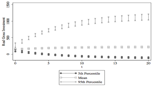
• Scenario 1: mean lagged investment, market value and capital stock held at their 95th percentiles,
• Scenario 2: all variables held at their means,
• Scenario 3: mean lagged investment, market value and capital stock held at their 5th percentiles.

We can create a list object for the scen argument containing each of these scenarios with the following code:

# Create simulation scenarios
attach(grunfeld)
Scen1 <- data.frame(InvestLag = mean(InvestLag,
                                 na.rm = TRUE),
                    mvalue = quantile(mvalue, 0.95),
                    kstock = quantile(kstock, 0.95))
Scen2 <- data.frame(InvestLag = mean(InvestLag,
                                 na.rm = TRUE),
                    mvalue = mean(mvalue),
                    kstock = mean(kstock))
Scen3 <- data.frame(InvestLag = mean(InvestLag,
                                 na.rm = TRUE),
                    mvalue = quantile(mvalue, 0.05),
                    kstock = quantile(kstock, 0.05))
detach(grunfeld)

# Combine into a single list
ScenComb <- list(Scen1, Scen2, Scen3)

In this example we won't introduce shocks, so now we run our simulations:

Sim1 <- dynsim(obj = M1, ldv = 'InvestLag',
                scen = ScenComb, n = 20)

This took 1000 draws of the coefficients to produce 20 dynamic simulation iterations for each of the three scenarios. In the resulting Sim1 object we have retained the middle 95% and 50%. We will return to presenting and exploring the contents of Sim1 later.

Dynamic simulation with shocks

Now let's include fitted shock values. In particular, let's see how a company with capital stock in the 5th percentile is predicted to change its gross investment when its market value experiences shocks compared to a company with capital stock in the 95th percentile. We will use market values for the first company in the grunfeld data set over the first 15 years as the shock values. To create the shock data use the following code:

# Keep only the mvalue for the first company 
# for the first 15 years
grunfeldsub <- subset(grunfeld, company == 1)
grunfeldshock <- grunfeldsub[1:15, 'mvalue']

# Create data frame for the shock argument
grunfeldshock <- data.frame(times = 1:15,
                    mvalue = grunfeldshock)

Now we can simply add grunfeldshock to the dynsim shocks argument.

Sim2 <- dynsim(obj = M1, ldv = 'InvestLag',
               scen = ScenComb, n = 15,
               shocks = grunfeldshock)

Now we can simply add grunfeldshock to the dynsim shocks argument.

Sim3 <- dynsim(obj = M1, ldv = 'InvestLag',
               scen = ScenComb, n = 15,
               shocks = grunfeldshock)

Plotting simulations

Probably the easiest and most effective way to communicate your dynsim simulation results is with the package’s built-in plotting capabilities. These are accessed with the dysnsimGG command. Let’s start by plotting the simulations from our basic model. In an earlier example we put these results into Sim1. Using dynsimGG's default settings we can plot the simulations with the following code:

dynsimGG(Sim1)

We can make a number of aesthetic changes. For example, we can re-title the legend using the leg.name argument and change the legend values by adding a vector of the desired label names in the order of our scenarios using the leg.labels argument. We can also change the color palette using the color argument. Let’s use the 'orange-red' palette denoted by OrRd. Finally, we can change the y-axis label with the ylab argument so that it is more descriptive.

# Create legend labels vector
Labels <- c('95th Percentile', 'Mean', '5th Percentile')

# Plot
dynsimGG(Sim1, leg.name = 'Scenarios',
         leg.labels = Labels, color = 'OrRd',
         ylab = 'Predicted Real Gross Investment\n')

Plotting simulations with shock variables is very similar to what we have already seen. The one major change we can make is to include a plot of one shock variable’s fitted values underneath the main plot. To do this simply use the shockplot.var argument to specify which variable to plot. Use the shockplot.ylab argument to change the y-axis label. For example:

dynsimGG(Sim2, leg.name = 'Scenarios', leg.labels = Labels,
            color = 'OrRd',
            ylab = 'Predicted Real Gross Investment\n',
            shockplot.var = 'mvalue',
            shockplot.ylab = 'Firm Value')

Similarly, we can plot the simulations from scenarios where market value shocks were interacted with capital stock. The code is accomplish this is almost identical to the code chunk we just saw. The only difference is that we use the Sim3 model object.

dynsimGG(Sim3, leg.name = 'Scenarios', leg.labels = Labels,
         color = 'OrRd',
         ylab = 'Predicted Real Gross Investment\n',
         shockplot.var = 'mvalue',
         shockplot.ylab = 'Firm Value')

Install

dynsim for R is available on CRAN.

You can also easily install the latest development version with devtools package:

devtools::install_github('christophergandrud/dynsim')